
Simple ODE
## =============================================================================
## R-Code to solve example 3.1.2 from the book
## K. Soetaert, J. Cash and F. Mazzia, 2012.
## Solving differential equations in R. UseR, Springer, 248 pp.
## http://www.springer.com/statistics/computational+statistics/book/978-3-642-28069-6.
## implemented by Karline Soetaert
## =============================================================================

## A simple ordinary differential equation model

a    <- -8/3 ; b <- -10; c <- 28
yini <- c(X = 1, Y = 1, Z = 1)

Lorenz <- function (t, y, parms) {
 with(as.list(y), {
    dX <- a * X + Y * Z
    dY <- b * (Y - Z)
    dZ <- -X * Y + c * Y - Z
    list(c(dX, dY, dZ))
 })
}

times <- seq(from = 0, to = 100, by = 0.01)
out   <- ode(y = yini, times = times, func = Lorenz, parms = NULL)

plot(out, lwd = 2)

library(plot3D)
pm <- par (mar = c(1, 1, 1, 1))
lines3D(out[,"X"], out[,"Y"], out[,"Z"], colkey = FALSE,
   colvar = out[,"Z"], bty = "f", main = "butterfly",
   phi = 0)
par (mar = pm)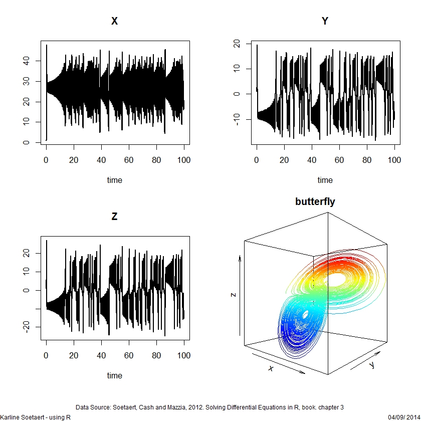
ODE events
## =============================================================================
## R-Code to solve example 3.4.1.2 from the book
## K. Soetaert, J. Cash and F. Mazzia, 2012.
## Solving differential equations in R. UseR, Springer, 248 pp.
## http://www.springer.com/statistics/computational+statistics/book/978-3-642-28069-6.
## implemented by Karline Soetaert
## =============================================================================

## An ordinary differential equation model with events

b    <- 0.6
yini <- c(blood = 0)

pharmaco2 <- function(t, blood, p) {
  dblood <-  - b * blood
  list(dblood)
}

injectevents <- data.frame(var = "blood",
                          time =  0:20,
                          value = 40,
                          method = "add")
head(injectevents, n=3)

times <- seq(from = 0, to = 10, by = 1/24)

out2 <- ode(func = pharmaco2, times = times, y = yini,
           parms = NULL, method = "impAdams",
           events = list(data = injectevents))

plot(out2, lwd = 2)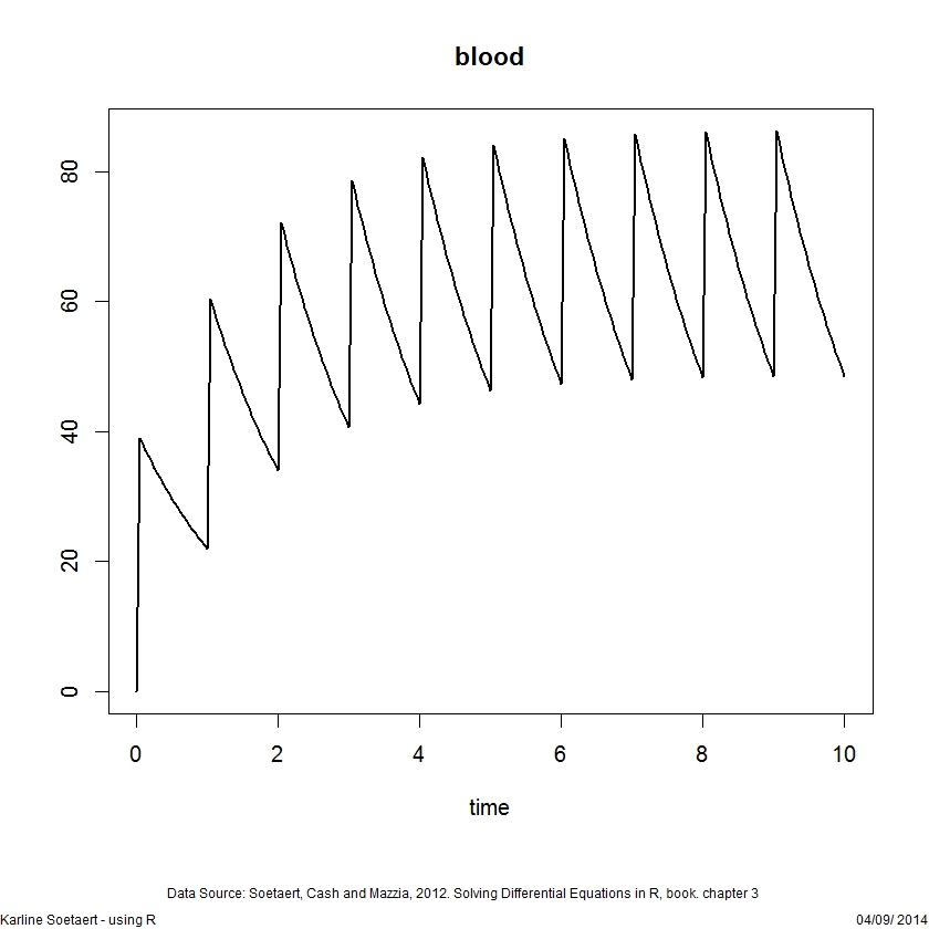
ODE forcings
## =============================================================================
## R-Code to solve example 3.3.2 from the book
## K. Soetaert, J. Cash and F. Mazzia, 2012.
## Solving differential equations in R. UseR, Springer, 248 pp.
## http://www.springer.com/statistics/computational+statistics/book/978-3-642-28069-6.
##
## An ordinary differential equation model with forcing functions
## The ozone model  - needs file "light.rda"
## implemented by Karline Soetaert
## =============================================================================

library (deSolve)

load(file = "light.rda")   # contains data.frame Light
head(Light, n = 4)

irradiance <- approxfun(Light)
irradiance(seq(from = 0, to = 1, by = 0.25))
k3 <- 1e-11; k2 <- 1e10; k1a <- 1e-30
k1b <- 1; sigma <- 1e11
yini <- c(O = 0, NO = 1.3e8, NO2 = 5e11, O3 = 8e11)

chemistry <- function(t, y, parms) {
  with(as.list(y), {

    radiation <- irradiance(t)
    k1  <- k1a + k1b*radiation

    dO   <-  k1*NO2 - k2*O
    dNO  <-  k1*NO2        - k3*NO*O3 + sigma
    dNO2 <- -k1*NO2        + k3*NO*O3
    dO3  <-           k2*O - k3*NO*O3
    list(c(dO, dNO, dNO2, dO3), radiation = radiation)
  })
}

times <- seq(from = 8/24, to = 5, by = 0.01)
out <- ode(func = chemistry, parms = NULL, y = yini,
          times = times, method = "bdf")

plot(out, type = "l", lwd = 2, las = 1)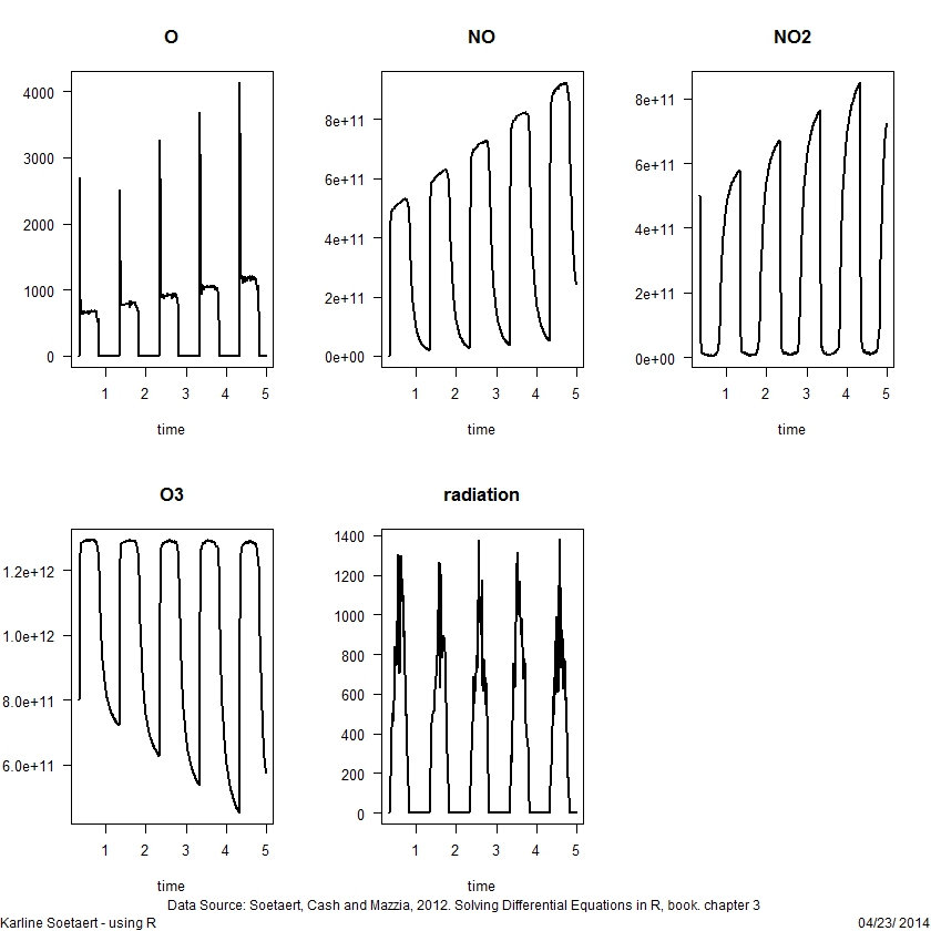
ODE roots
## =============================================================================
## R-Code to solve example 3.4.2 from the book
## K. Soetaert, J. Cash and F. Mazzia, 2012.
## Solving differential equations in R. UseR, Springer, 248 pp.
## http://www.springer.com/statistics/computational+statistics/book/978-3-642-28069-6.
## implemented by Karline Soetaert
## =============================================================================

## An ordinary differential equation model with root and events
library(deSolve)
yini  <- c(height = 0, velocity = 10)

ball <- function(t, y, parms) {
  dy1 <- y[2]
  dy2 <- -9.8

  list(c(dy1, dy2))
}

rootfunc <- function(t, y, parms) y[1]

eventfunc <- function(t, y, parms) {
 y[1] <- 0
 y[2] <- -0.9*y[2]
 return(y)
}

times <- seq(from = 0, to = 20, by = 0.01)
out <- ode(times = times, y = yini, func = ball,
             parms = NULL, rootfun = rootfunc,
             events = list(func = eventfunc, root = TRUE))

plot(out, which = "height", lwd = 2,
    main = "bouncing ball", ylab = "height")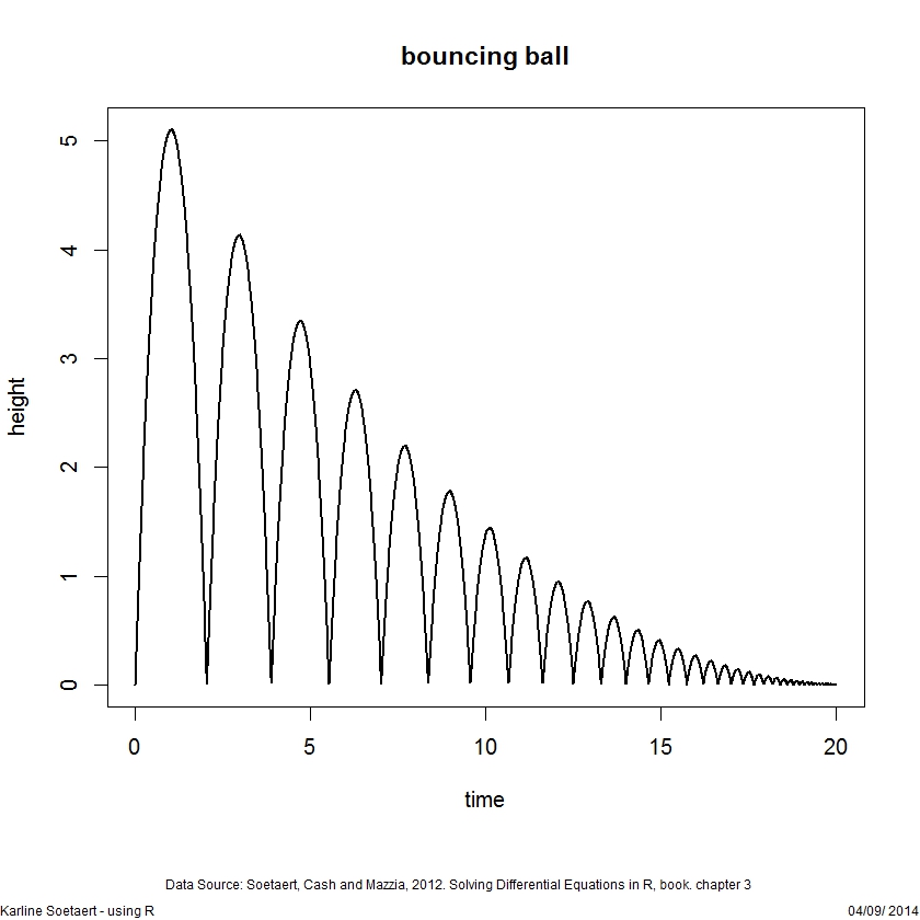
DAE
## =============================================================================
## R-Code to solve example 5.5.1 from the book
## K. Soetaert, J. Cash and F. Mazzia, 2012.
## Solving differential equations in R. UseR, Springer, 248 pp.
## http://www.springer.com/statistics/computational+statistics/book/978-3-642-28069-6.
## implemented by Karline Soetaert
## =============================================================================

## A differential algebraic equation model
library(deSolve)

Caraxis <- function(t, y, dy, parms) {
 with(as.list(y), {
   f <- rep(0, 10)
   yb <- r * sin(w * t)
   xb <- sqrt(L^2  - yb^2)
   Ll <- sqrt(xl^2 + yl^2)
   Lr <- sqrt((xr - xb)^2 + (yr - yb)^2)
   f[1:4] <- y[5:8]
   f[5] <- 1/k*((L0-Ll)*xl/Ll + lam1*xb + 2*lam2*(xl-xr))
   f[6] <- 1/k*((L0-Ll)*yl/Ll + lam1*yb + 2*lam2*(yl-yr)) -g
   f[7] <- 1/k*((L0-Lr)*(xr - xb)/Lr    - 2*lam2*(xl-xr))
   f[8] <- 1/k*((L0-Lr)*(yr - yb)/Lr    - 2*lam2*(yl-yr)) -g
   f[9] <- xb * xl + yb * yl
   f[10]<- (xl - xr)^2 + (yl - yr)^2 - L^2

   delt       <- dy - f
   delt[9:10] <- -f[9:10]

   list(delt)
 })
}

eps <- 0.01; M <- 10; k <- M * eps * eps/2
L <- 1; L0 <- 0.5; r <- 0.1; w <- 10; g <- 9.8

yini <- c(xl = 0,     yl = L0, xr = L,     yr = L0,
         ul = -L0/L, vl = 0,  ur = -L0/L, vr = 0,
         lam1 = 0, lam2 = 0)

library(deTestSet)
rootfun <- function (dyi, y, t)
  unlist(Caraxis(t, y, dy = c(dyi, 0, 0),
        parms = NULL)) [1:8]

dyini <- multiroot(f = rootfun, start = rep(0,8),
                  y = yini, t = 0)$root
(dyini <- c(dyini, 0, 0))
Caraxis(t = 0, yini, dyini, NULL)

index <- c(4, 4, 2)
times <- seq(from = 0, to = 3, by = 0.01)
out <- mebdfi(y = yini, dy = dyini, times = times,
             res = Caraxis, parms = parameter, nind = index)

par(mar = c(4, 4, 3, 2))
plot(out, lwd = 2, mfrow = c(4,3))
plot(out[,c("xl", "yl")], xlab = "xleft", ylab = "yleft",
    type = "l", lwd = 2)
plot(out[,c("xr", "yr")], xlab = "xright", ylab = "yright",
    type = "l", lwd = 2)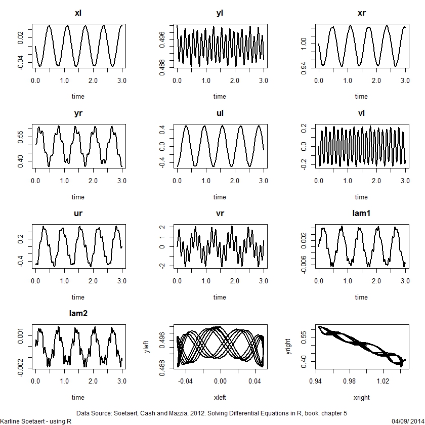
DAE mass
## =============================================================================
## R-Code to solve example 5.6.1 from the book
## K. Soetaert, J. Cash and F. Mazzia, 2012.
## Solving differential equations in R. UseR, Springer, 248 pp.
## http://www.springer.com/statistics/computational+statistics/book/978-3-642-28069-6.
##
## A DAE model, solved in linearly implicit form
## The transistor amplifier
## implemented by Karline Soetaert
## =============================================================================

library(deSolve)

Transistor <- function(t, u, du, pars) {
  delt <- vector(length = 8)
   uin  <- 0.1 * sin(200 * pi * t)
   g23  <- beta * (exp( (u[2] - u[3]) / uf) - 1)
   g56  <- beta * (exp( (u[5] - u[6]) / uf) - 1)

   delt[1] <- (u[1] - uin)/R0
   delt[2] <- u[2]/R1 + (u[2]-ub)/R2 + (1-alpha) * g23
   delt[3] <- u[3]/R3 - g23
   delt[4] <- (u[4] - ub) / R4 + alpha * g23
   delt[5] <- u[5]/R5 + (u[5]-ub)/R6 + (1-alpha) * g56
   delt[6] <- u[6]/R7 - g56
   delt[7] <- (u[7] - ub) / R8 + alpha * g56
   delt[8] <- u[8]/R9
   list(delt)
}

ub <- 6; uf <- 0.026; alpha <- 0.99; beta <- 1e-6; R0 <- 1000
R1 <- R2 <- R3 <- R4 <- R5 <- R6 <- R7 <- R8 <- R9 <- 9000
C1 <- 1e-6; C2 <- 2e-6; C3 <- 3e-6; C4 <- 4e-6; C5 <- 5e-6

mass <- matrix(nrow = 8, ncol = 8, byrow = TRUE, data = c(
      -C1,C1, 0,  0,  0,  0,  0,  0,
      C1,-C1, 0,  0,  0,  0,  0,  0,
      0,  0,-C2,  0,  0,  0,  0,  0,
      0,  0,  0,-C3, C3,  0,  0,  0,
      0,  0,  0, C3,-C3,  0,  0,  0,
      0,  0,  0,  0,  0,-C4,  0,  0,
      0,  0,  0,  0,  0,  0,-C5, C5,
      0,  0,  0,  0,  0,  0, C5,-C5
))

yini <- c(0, ub/(R2/R1+1), ub/(R2/R1+1),
         ub, ub/(R6/R5+1), ub/(R6/R5+1), ub, 0)
names(yini) <- paste("u", 1:8, sep = "")

ind   <- c(8, 0, 0)
times <- seq(from = 0, to = 0.2, by = 0.001)

out <- radau(func = Transistor, y = yini, parms = NULL,
            times = times, mass = mass, nind = ind)

plot(out, lwd = 2, which = c("u1", "u4", "u5", "u8"))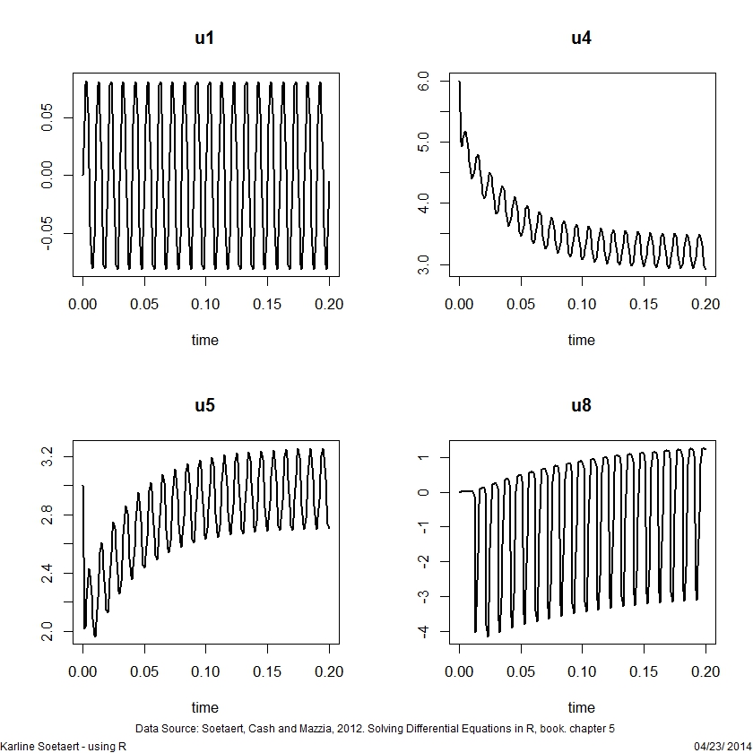
DDE
## =============================================================================
## R-Code to solve example 7.3 from the book
## K. Soetaert, J. Cash and F. Mazzia, 2012.
## Solving differential equations in R. UseR, Springer, 248 pp.
## http://www.springer.com/statistics/computational+statistics/book/978-3-642-28069-6.
## implemented by Karline Soetaert
## =============================================================================

## A delay differential equation model
library(deSolve)

mackey <- function(t, y, parms, tau) {
  tlag <- t - tau
  if (tlag <= 0)
    ylag <- 0.5
  else
    ylag <- lagvalue(tlag)
  dy <- 0.2 * ylag * 1/(1+ylag^10) - 0.1 * y
  list(dy = dy, ylag = ylag)
}

yinit <- 0.5
times <- seq(from = 0, to = 300, by = 0.1)

yout1 <- dede(y = yinit, times = times, func = mackey,
             parms = NULL, tau = 10)
yout2 <- dede(y = yinit, times = times, func = mackey,
             parms = NULL, tau = 20)

plot(yout1, lwd = 2, main = "tau=10",
    ylab = "y", mfrow = c(2, 2), which = 1)
plot(yout1[,-1], type = "l", lwd = 2, xlab = "y")
plot(yout2, lwd = 2, main = "tau=20",
    ylab = "y", mfrow = NULL, which = 1)
plot(yout2[,-1], type = "l", lwd = 2, xlab = "y")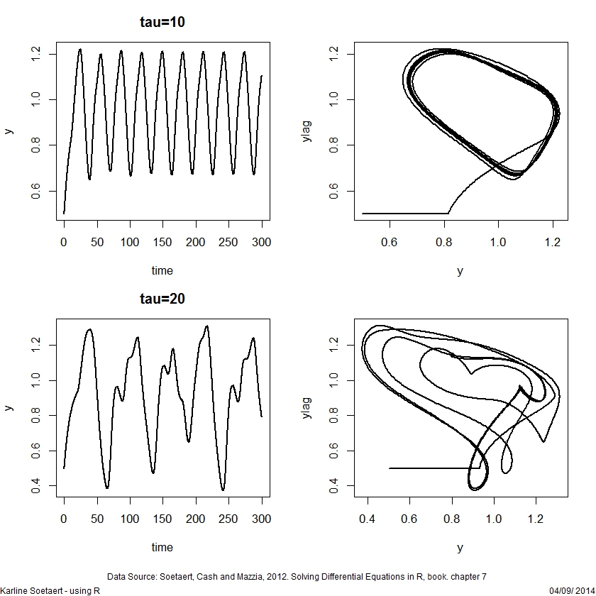
DDE events
## =============================================================================
## R-Code to solve example 7.6 from the book
## K. Soetaert, J. Cash and F. Mazzia, 2012.
## Solving differential equations in R. UseR, Springer, 248 pp.
## http://www.springer.com/statistics/computational+statistics/book/978-3-642-28069-6.
##
## A delay differential equation model
## Predator-prey with harvesting  - takes a while
## implemented by Karline Soetaert
## -----------------------------------------------------------------------------

library(deSolve)
LVdede <- function(t, y, p) {
 if (t > tau1) Lag1 <- lagvalue(t - tau1) else Lag1 <- yini
 if (t > tau2) Lag2 <- lagvalue(t - tau2) else Lag2 <- yini

 dy1 <- r * y[1] *(1 - Lag1[1]/K) - a*y[1]*y[2]
 dy2 <- a * b * Lag2[1]*Lag2[2] - d*y[2]

 list(c(dy1, dy2))
}

rootfun <- function(t, y, p)
  return(y[1] - Ycrit)

eventfun <- function(t, y, p)
  return (c(y[1] * 0.7, y[2]))

r <- 1; K <- 1; a <- 2; b <- 1; d <- 1; Ycrit <- 1.2*d/(a*b)
tau1 <- 0.2; tau2 <- 0.2

yini <- c(y1 = 0.2, y2 = 0.1)
times <- seq(from = 0, to = 200, by = 0.01)
yout <- dede(func = LVdede, y = yini, times = times,
           parms = 0, rootfun = rootfun,
           events = list(func = eventfun, root = TRUE))
attributes(yout)$troot [1:10]

plot(yout[,-1], type = "l")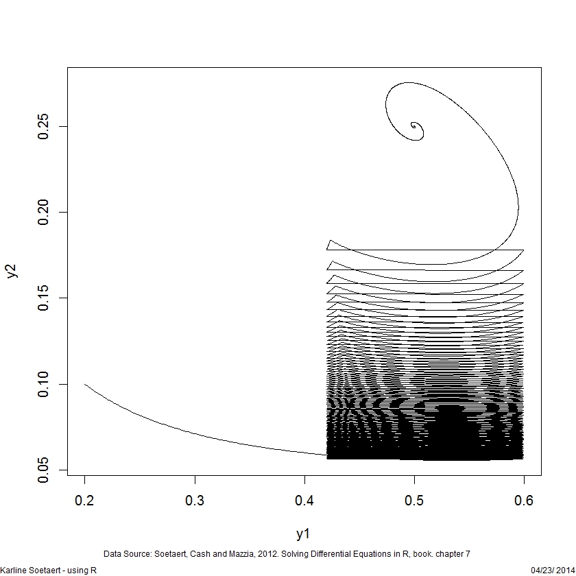
PDE
## =============================================================================
## R-Code to solve example 9.3.4 from the book
## K. Soetaert, J. Cash and F. Mazzia, 2012.
## Solving differential equations in R. UseR, Springer, 248 pp.
## http://www.springer.com/statistics/computational+statistics/book/978-3-642-28069-6.
## implemented by Karline Soetaert
## =============================================================================

## A 3-D partial differential equation model
library(deSolve)

Nx  <- 100
Ny  <- 100

xgrid <- setup.grid.1D(-7, 7, N=Nx)
ygrid <- setup.grid.1D(-7, 7, N=Ny)

x <- xgrid$x.mid
y <- ygrid$x.mid

sinegordon2D <- function(t, C, parms) {

   u <- matrix(nrow = Nx, ncol = Ny,
              data = C[1 : (Nx*Ny)])
   v <- matrix(nrow = Nx, ncol = Ny,
              data = C[(Nx*Ny+1) : (2*Nx*Ny)])

   dv <- tran.2D (C = u, C.x.up = 0, C.x.down = 0,
                 C.y.up = 0, C.y.down = 0,
                 D.x = 1, D.y = 1,
                 dx = xgrid, dy = ygrid)$dC - sin(u)
   list(c(v, dv))
}

peak <- function (x, y, x0 = 0, y0 = 0)
                 exp(-((x-x0)^2 + (y-y0)^2))
uini <- outer(x, y,
 FUN = function(x, y) peak(x, y, 2,2) + peak(x, y,-2,-2)
                    + peak(x, y,-2,2) + peak(x, y, 2,-2))
vini <- rep(0, Nx*Ny)

times <- 0:3
print(system.time(
out  <- ode.2D (y = c(uini, vini), times = times,
               parms = NULL, func = sinegordon2D,
               names = c("u", "v"),
               dimens = c(Nx, Ny), method = "ode45")
))

mr <- par(mar = c(0, 0, 1, 0))
image(out, main = paste("time =", times), which = "u",
     grid = list(x = x, y = y), method = "persp",
     border = NA, col = "grey",  box = FALSE,
     shade = 0.5, theta = 30, phi = 60, mfrow = c(2, 2),
     ask = FALSE)
par(mar = mr)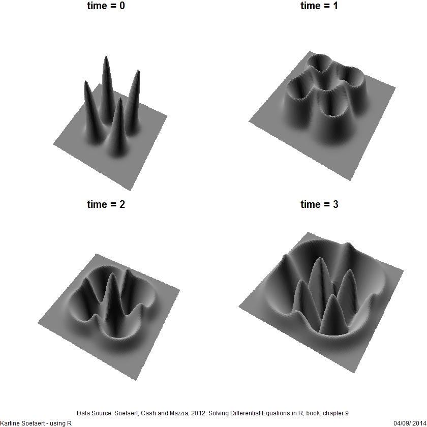
PDE imaginary
## =============================================================================
## R-Code to solve example 9.3.4 from the book
## K. Soetaert, J. Cash and F. Mazzia, 2012.
## Solving differential equations in R. UseR, Springer, 248 pp.
## http://www.springer.com/statistics/computational+statistics/book/978-3-642-28069-6.
## implemented by Karline Soetaert
## =============================================================================

## A partial differential equation model with complex numbers
library(deSolve)

alf <- 0.5
gam <- 1

Schrodinger <- function(t, u, parms) {
   du <- 1i * tran.1D (C = u, D = 1, dx = xgrid)$dC  +
                1i * gam * abs(u)^2 * u
   list(du)
}
N     <- 300
xgrid <- setup.grid.1D(-20, 80, N = N)
x     <- xgrid$x.mid

c1  <- 1
c2  <- 0.1

sech    <- function(x) 2/(exp(x) + exp(-x))
soliton <- function (x, c1)
  sqrt(2*alf/gam) * exp(0.5*1i*c1*x) * sech(sqrt(alf)*x)

yini <- soliton(x, c1) + soliton(x-25, c2)

times <- seq(0, 40, by = 0.1)
print(system.time(
 out <- ode.1D(y = yini, parms = NULL, func = Schrodinger,
              times = times, dimens = 300, method = "adams")
))

image(abs(out), grid = x, ylab = "x", main = "two solitons",
  legend = TRUE)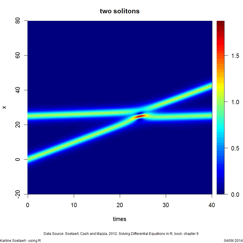
BVP
## =============================================================================
## R-Code to solve example 11.3 from the book
## K. Soetaert, J. Cash and F. Mazzia, 2012.
## Solving differential equations in R. UseR, Springer, 248 pp.
## http://www.springer.com/statistics/computational+statistics/book/978-3-642-28069-6.
## implemented by Karline Soetaert
## =============================================================================

## A boundary value problem
library(bvpSolve)
swirl <- function (t, Y, eps)  {
  with(as.list(Y),
    list(c((g*f1 - f*g1)/eps,
          (-f*f3 - g*g1)/eps))
      )
}

eps  <- 0.001
x    <- seq(from = 0, to = 1, length = 100)
yini <- c(g = -1, g1 = NA, f = 0, f1 = 0, f2 = NA, f3 = NA)
yend <- c(1, NA, 0, 0, NA, NA)
Soltwp <- bvptwp(x = x, func = swirl, order = c(2, 4),
                 par = eps, yini = yini, yend = yend)

pairs(Soltwp, main = "swirling flow III, eps=0.001",
  pch = 16, cex = 0.5)

diagnostics(Soltwp)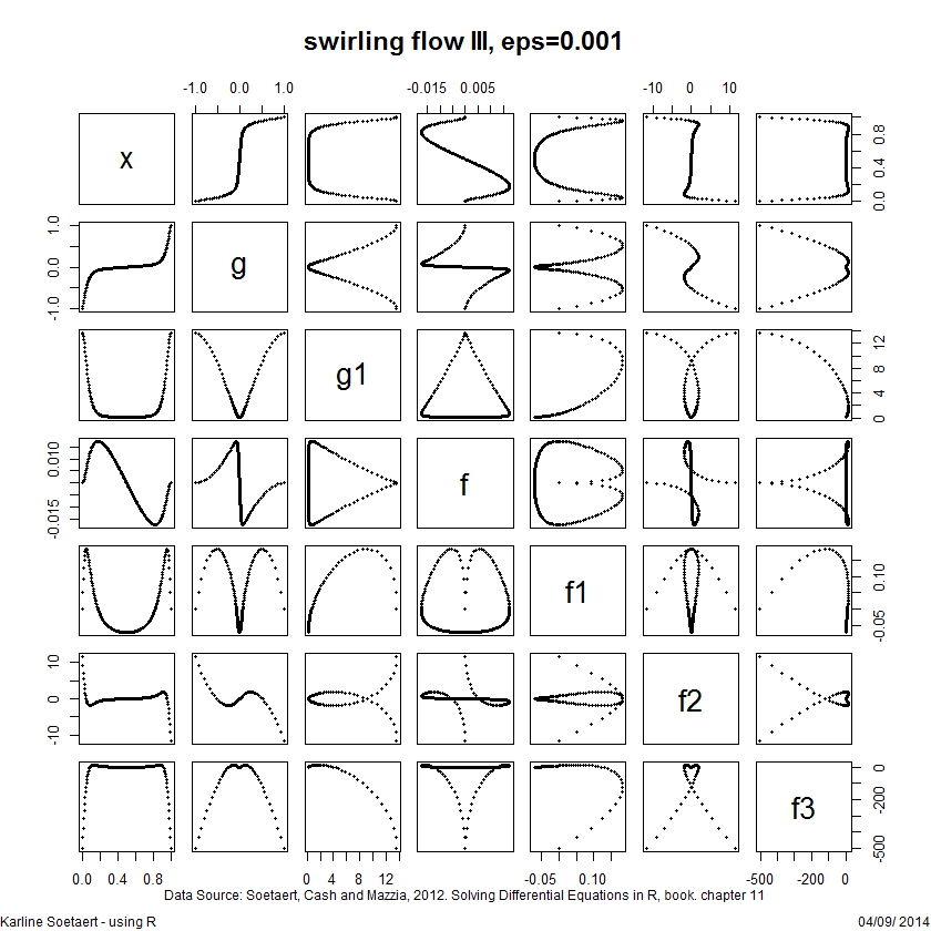
BVP reaction transport
## =============================================================================
## R-Code to solve example 11.9 from the book
## K. Soetaert, J. Cash and F. Mazzia, 2012.
## Solving differential equations in R. UseR, Springer, 248 pp.
## http://www.springer.com/statistics/computational+statistics/book/978-3-642-28069-6.
## implemented by Karline Soetaert
## =============================================================================

## Steady-state solution of a reaction-transport problem
library(ReacTran)

N    <- 1000
Grid <- setup.grid.1D(N = N, L = 100000)
v <- 1000; D <- 1e7; O2s <- 300
NH3in <- 500; O2in <- 100; NO3in <- 50
r <- 0.1; k <- 1.; p <- 0.1

Estuary <- function(t, y, parms)  {
 NH3 <- y[1:N]
 NO3 <- y[(N+1):(2*N)]
 O2  <- y[(2*N+1):(3*N)]
 tranNH3<- tran.1D (C = NH3, D = D, v = v,
             C.up = NH3in, C.down = 10,  dx = Grid)$dC
 tranNO3<- tran.1D (C = NO3, D = D, v = v,
             C.up = NO3in,  C.down = 30,  dx = Grid)$dC
 tranO2 <- tran.1D (C = O2 , D = D, v = v,
             C.up = O2in, C.down = 250, dx = Grid)$dC

 reaeration <- p * (O2s - O2)
 r_nit      <- r * O2 / (O2 + k) * NH3

 dNH3    <- tranNH3 - r_nit
 dNO3    <- tranNO3 + r_nit
 dO2     <- tranO2  - 2 * r_nit + reaeration

 list(c(  dNH3, dNO3, dO2 ))
}

print(system.time(
std <- steady.1D(y = runif(3 * N), parms = NULL,
             names=c("NH3", "NO3", "O2"),
             func = Estuary, dimens = N,
             positive = TRUE)
))

NH3in <- 100
std2 <- steady.1D(y = runif(3 * N), parms = NULL,
             names=c("NH3", "NO3", "O2"),
             func = Estuary, dimens = N,
             positive = TRUE)

plot(std, std2, grid = Grid$x.mid, ylab = "mmol/m3", lwd = 2,
     xlab = "m", mfrow = c(1,3), col = c("black", "red"))
legend("bottomright", lty = 1:2, title = "NH3in", lwd = 2,
      legend = c(500, 100), col = c("black", "red"))