
Linear equations
An important part of our research deals with food web models, which are typically written as a set of linear equations comprising a few hundred unknowns.
When we started this research, our main challenge was not to solve these equations, but to create them!
The way we work is as follows: first the model problem is formulated in text files in a way that is natural and comprehensible. This input is then converted, using functions in the LIM package, into linear equality and inequality conditions. These are then solved either by least squares or by linear programming techniques, as implemented in the package limSolve. After that, we can use package NetIndices to calculate some characteristics from the quantified networks.
We use these packages for our food web models, or to create mass balanced budgets in biogeochemical applications, but they are also suited for flux balance analysis or even to solve more general (linear) operational research problems. Here you will find one example of each, consisting of the input file, and the R-code to solve the problem.
R code
## =============================================================================
## The Gulf of Riga *SPRING* planktonic food web
## =============================================================================

library(LIM)

# Read data and create the LIM structure with the equations, variables, ..
LIMRigaSpring <- Setup(file = "RigaSpring.input")

# Create the flow matrix and plot it
rigaSpring <- Flowmatrix(LIMRigaSpring)
plotweb(rigaSpring, main = "Gulf of Riga planktonic food web, spring",
        sub = "mgC/m3/day")

# Create and plot ranges of flows and of variables
Plotranges(LIMRigaSpring, lab.cex = 0.7,
        main = "Gulf of Riga planktonic food web, spring, Flowranges")
Plotranges(LIMRigaSpring, type = "V", lab.cex = 0.7,
        main = "Gulf of Riga planktonic food web, spring, Variable ranges")
Input file
R code
## =============================================================================
## A 0-dimensional sediment coupled C, N, O, P model
## =============================================================================

require(LIM)
reaction.lim <-Setup("Reaction.input")

# parsimonious solution
pars   <- Ldei(reaction.lim)

# ranges
ranges <- Xranges(reaction.lim, ispos = FALSE)
data.frame(ranges, pars = pars$X)

# take a random sample of valid solutions
xs <- Xsample(reaction.lim, jmp = 10, iter = 500)

panel.hist <- function(x, ...)  {
    usr <- par("usr"); on.exit(par(usr))
    par(usr = c(usr[1:2], 0, 1.5) )  #redefine y-axis; x-axis stays the same
    h <- hist(x, plot = FALSE)
    breaks <- h$breaks; nB <- length(breaks)
    y <- h$counts; y <- y/max(y)
    rect(breaks[-nB], 0, breaks[-1], y, col="grey", ...)
}

xs <- xs[, -(7:9)]                    #remove constant rates

pairs(xs, upper.panel = NULL, diag.panel = panel.hist,
      pch  =".", cex = 2, main = "Reaction network")

Mean <- colMeans(xs)
Sd   <- apply(xs, 2, sd)
data.frame(mean = Mean, sd = Sd)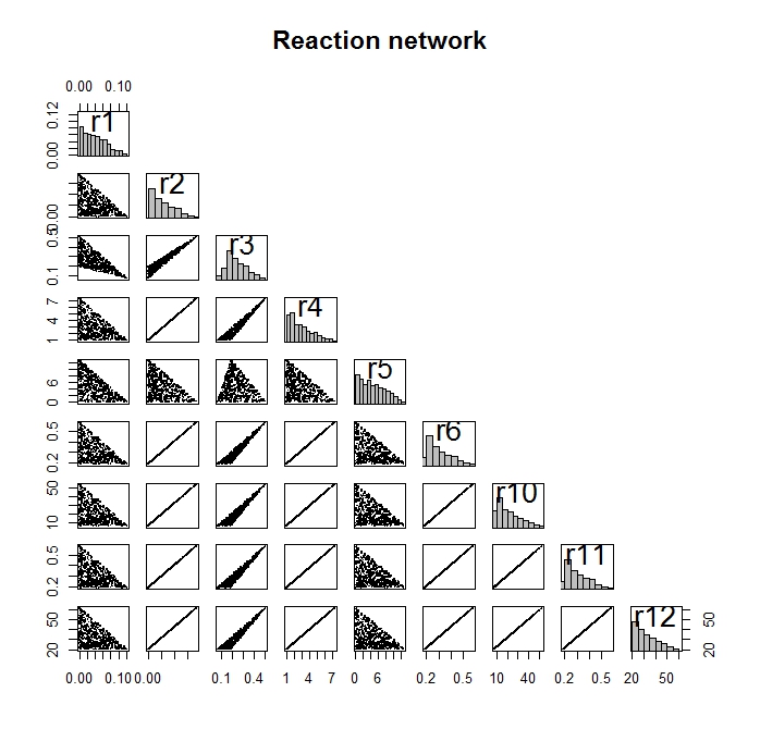
Input file
R code
## ===================================
## R code to solve the blending model
## ===================================

require(LIM)
LIMBlending <- Setup("Blending.input")
print(Linp(LIMBlending))